Peak Force Kelvin Probe of Polyphase Polymers

In this example we look at polyphase polymers with PeakForce Kelvin probe microscopy. This sample consists of polystyrene (PS) with polydimethylsiloxane (PDMS) inclusions. These inclusions are soft, with an elastic modulus of 2.5-3.5 MPa, while the surround polystyrene is around 3 GPa.

This is a great sample for contrast in mechanical measurement techniques like PeakForce QNM, force volume, and so on. And it is a good representative of a soft sample that is well suited to PeakForce imaging where the peak normal force is known and controlled with minimal shear force. This allows for imaging under different peak normal forces, which can lead to different surface structures just due to deformation of the surface and interaction with subsurface structures.

The top image is a height image taken with a peak normal force of 5 nN using a fairly stiff probe, a silicon SCM-PIT which has a spring constant of around 3 nN/nm. Deflection sensitivity was calibrated on sapphire, and the spring constant was estimated through thermal tuning to be around 2.1 nN/nm. This is stiff enough of a probe that the Sader method is more appropriate.

Since the SCM-PIT is coated with PtIr for EFM and KPFM, it was possible to do KPFM to image the surface potential. Initially this sample was chosen to calibrate the probe radius to  simultaneously do QNM and KPFM, to correlate both nanomechanical properties and surface potential properties of a different sample.

But-- why not KPFM on a soft biphasic polymer?

The bottom image is the raw PeakForce KPFM channel. The lift was 50 nm with a scan-rate of 0.1 Hz. A three hour image! What is immediately obvious is that the PDMS domains have a surface potential some 50-70 mV higher than the PS. There is also a potential "plateau" across the top left of the image, and athese little specs on some of the PS inclusions are clearly hitchhikers, contaminants, and they have a surface potential of 200-400 mV above the neighboring PS background.

KPFM and EFM of Exfoliated HOPG

In this demonstration, a piece of HOPG was grounded on the stage of the Bruker Icon using graphitic paint. An SCM-PIT probe was used to perform both PeakForce KPFM (Kelvin probe force microscopy) and EFM (electric force microscopy) on a region of the sample that presented broken edges of the exfoliated HOPG lamella.

The first image shows the height image taken in PeakForce mode. A normal force of about 10 nN was used, and even this is causing some disturbance of the graphitic lamella. Some of the sheets seem to come in multiple copies. This is actually not the result of a tip-artifact, as the effect goes away when switching to a lower peak force set-point, or when switching to tapping AFM in order to subsequently do EFM. The intermittent normal forces the sample sees in tapping AFM are much smaller than the 10 nN peak force used here. A larger peak force set-point was used only to help track the drastic topographic relief in this particular sample. This perturbation of the graphite lamella by 10 nN of peak normal force shows how flexible and loosely coupled they are.

The next image was taken in tapping AFM in lift mode to facilitate EFM imaging. EFM is an imaging mode that applies scanning interleave. There is one pass across the sample to image sample morphology, and then a second pass along the same trace-retrace. One can do anything one likes with the interleave pass. Take a second image with any change of parameters one likes from a different set of gains and set-point to a probe-sample bias. In this case the probe is lifted 100 nm above the surface of the sample and changes in probe amplitude and phase are detected. As in MFM (magnetic force microscopy) the amplitude change says something about the magnitude of an electric field gradient, and a phase change says something about its sign-- whether it is repulsive or attractive as seen by the probe.


The results were are quite curious. HOPG is quite a good conductor, and the sample was well grounded using graphitic paint. It is interesting that any EFM signal is seen whatsoever given that it is not biased. The signal is small. There is only about a 0.5 nm amplitude change across the whole image region, but it clearly correlates with the edges of the lamella. The edges are the source of a gradient.

Like MFM, EFM can be a bit difficult to interpret as one is probing an electric field gradient, and unless the geometry is of planar ferroelectric domains, or a planar fabricated device, it is often not clear what is causing these gradients: geometry, gradient in the potential creating the electric field, dielectric gradients. All that can be determined is that the magnitude of the EFM signal (i.e. the electric field gradient) is larger near the edges of the lamella, and trails off from there.

The EFM phase signal is, like the amplitude signal, very weak. About a half a degree of phase change over the whole image field. The signal is limited to the broken lamella edges and the rest of the lamellae are generally neutral in signal. This would seem to indicate a repulsive electric field gradient-- but it is harder to know what an electric field gradient says about the electric field itself. That is particularly the case in EFM where there are capacitive as well as charge effects that produce the EFM signal.

The last image is the KPFM which was done in PeakForce mode. This is actually measuring the surface potential in the interleave scan. What we see is an accumulation of potential on the broken edges of the lamella. Quite a small signal, a few 10's mV, but definitely consistent, repeatable, and correlating with the edges of the broken lamella. Given that this sample is conducting and well grounded with no applied potential to the probe or stage, this is surplus surface charge from the beaking of bonds?

Image Sectioning: Collagen D-bands (Part 1)

Images can be sectioned using the sectioning tool. In this case an image of human collagen was taken with PeakForce tapping. The image was flattened to remove large scale spatial relationships not related to the structure of individual collagen fibrils.

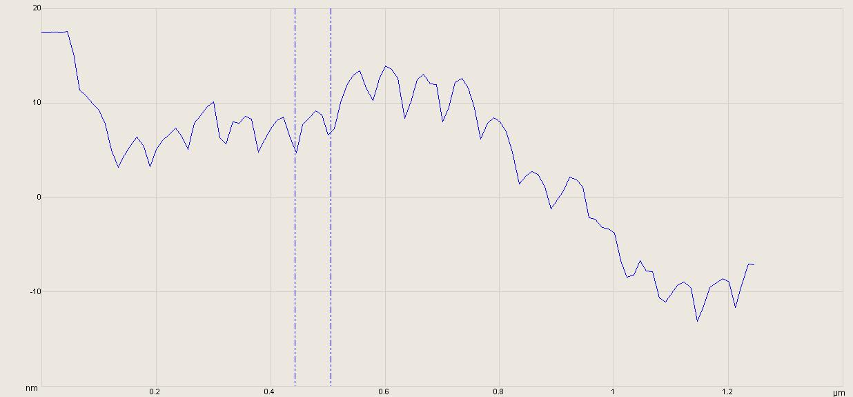
The D-bands arising from the staggering of tropocollagen structural units is clearly visualized on individual collagen fibrils. By drawing the sectioning tool across individual fibers, an effective digital cross section of the fiber along that line is produced. In this case the spacing between two specific bands is found to be 54 nm.  While the D-band period is a function of such environmental parameters as hydration, this is far less than the expected 67 nm seen in TEM of stained fibrils.

Application of the sectioning tool can be problematic as measurements are then biased according to the operator's selection of targets and placement of the dimensioning cursors. It is human nature of select features that are the least ambiguous and simplest to dimension by interacting with the image. As an example in this case I chose to section a long fiber in a cluster of long fibers. Removing operator bias would require a sampling methodology which covered more of the image field, including less "attractive" looking fibers, and statistically combining these measurements.

Human Collagen: PeakForce Tapping

The primary advantage of tapping AFM is that it is a non-contact AFM technique. While it "taps" on the sample surface, the tapping is intermittent and as such there is minimum shear force. This is ideal in imaging soft materials, including biological systems, as significant shear forces modify the sample surface while it is being imaged.

That tapping is generally done at the resonant frequency of the probe. A stiff silicon tapping probe has a resonant frequency on the order of 300 kHz, and so a tapping frequency just below resonance is selected for tapping AFM. Constraining the tapping causes the probe frequency to increase, and this will cause the probe frequency to move towards resonance not off resonance.

While this mode of imaging produces minimal shear force, one disadvantage is that it produces an indeterminate maximum normal force. While one can image in soft tapping mode by reducing the tapping amplitude, it is a non-trivial task to estimate the maximum peak normal force in tapping AFM. It is sometimes also desirable to know the maximum force exerted on a sample to quantitate sample deformation.

Bruker's PeakForce tapping combines the best of tapping and contact AFM imaging modes. What it does is perform complete force curves at 1-2 kHz at every image point. The force curve is triggered at the maximum applied normal force according to these force curves, and it is this "PeakForce" that is the set-point or parameter maintained constant during imaging. The second image, borrowed from Bruker, shows force curves as a function of time and position, and the PeakForce set-point is point C on both curves. A further innovation is ScanAsyst technology which dynamically and intelligently monitors and optimizes the scan rate, PeakForce set-point, gains, and Z-limit to produce the best image quality.

In this image human collagen from cadaver skin was imaged using a ScanAsyst Air probe in ScanAsyst mode. This image of a fairly soft biological specimen was imaged with little operator interaction beyond aligning the scanner and focusing on the sample. An additional advantage of the PeakForce tapping imaging mode is that force curves are available at every image point, and these can be used to perform nanomechanical measurements-- what is called PeakForce QNM.